
In this blog post, I briefly discuss some fundamental issues with OpenFOAM, preCICE and ANSYS for fluid-structure interaction (FSI) problems. This blog post is for you if you are interested in knowing why you often have to use smaller time steps when you run FSI simulations in OpenFOAM and ANSYS.
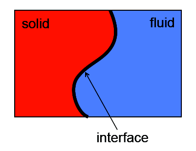
In FSI problems, fluid and solid domains interact with each other at the fluid-solid interface, see Figure 1. At the interface, we have two important conditions:
(i) Kinematic constraint: Requires that the velocity of the fluid (Vf) and the velocity of the solid (Vs) at the interface are the same. That is, the fluid moves at the same velocity as the velocity of the solid boundary. Thus,
Vs = Vf.
(ii) Traction equilibrium: Ensures the equilibrium of tractions at the interfaces. In the absence of surface tension, this is equivalent to the statement that the force on the solid (Fs) is exactly equal to the force exerted by the fluid (Ff) but in the opposite direction. That is,
Fs = –Ff.
Note: Traction equilibrium also extends to moments.
When simulating the FSI problems, the solid problem is solved with force exerted by the fluid as the Neumann boundary condition and the fluid problem is solved using the velocity of the solid as the Dirichlet boundary condition. This is the typical approach followed for FSI problems except for immersed boundary methods where the coupling is through body force.
However, ANSYS system coupling passes forces to the solid solver and displacements (instead of velocities) to the fluid solver. This is the same with OpenFOAM and preCICE. While we do need the displacement field of the solid boundary to update the fluid domain, we also need the velocities on the boundaries to use as the boundary conditions. If the velocities are not passed to the fluid domain, they are approximated, typically using first-order finite difference approximation.
While calculating the velocities using first-order finite difference approximation of displacements is a straightforward choice, it has some serious consequences. First and foremost, the velocity field at the moving boundary is approximated; this introduces an unnecessary error that converges linearly. Moreover, such a velocity field is not consistent with the velocity of the solid domain in every case, e.g. Newmark-beta method, HHT-alpha method, CH-alpha method, etc., except when the time integration scheme used for the solid problem is the backward Euler method. As the velocity boundary condition is (often) not correct, this error propagates into the subsequent solution in the fluid domain and the corresponding forces exerted on the solid domain. This is why one must use ridiculously smaller time steps when simulating FSI problems with OpenFOAM, ANSYS and preCICE, resulting in a significant increase in computational cost.
Although it is possible to achieve second-order accuracies just with displacements using second-order finite difference approximation, this is not equal to the velocity of the solid, making the velocity boundary condition in the CFD problem inconsistent with that of the solid boundary.
It is well understood that second-order and higher-order partitioned approaches have narrow stability limits when it comes to FSI problems. For challenging FSI problems involving thin lightweight structures, first-order schemes are the only choice, and we must use relaxation parameters to improve stability and convergence. This is perfectly fine! However, it is difficult to understand the rationale behind calculating the velocities, which are crucial BCs in CFD problems, using first-order approximations, as it is inconsistent with the solid velocity and introduces additional errors resulting in increased computational cost, while this information (velocity field) is readily available from the solid solver.
